One-way relationships

Posted by voracity on 1 April 2024, 8:00 pm

Let’s break down how subjective randomness allows us to cut out all other influences. Remember that our definition of subjective randomness had 3 parts: 1) sensitivity to conditions (or influences); 2) non-repetition of conditions; and 3) a lack of knowledge of the conditions. In this post, we’ll look at just part 1 of this definition.

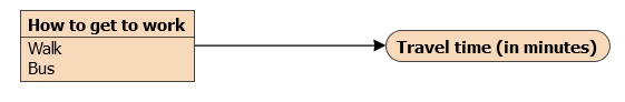
In posts gone by, we explored how we could estimate the causal effect of how we get to work on travel time without pesky confounders messing up our measurements. We came up with a list of possible confounders, things that could affect both our choice of how to get to work and travel time. Including these in our causal model made it look like this:

Basing our choice on a coin toss would cut out the influences on how we get to work, which would also remove the confounding. But wouldn’t some of these influences, like mood and energy, also affect the coin toss anyway? So perhaps the new causal model would be something like this:

All the influences into how to get to work have been cut by the green arrow. The black arrows that remain are pretty straightforward. For example, it’s reasonable to say that the more energy you have, the less time it will take you to walk to work. But those grey arrows are a bit odd. We know mood and energy will affect the coin toss outcome, but we’re a bit fuzzy on how. For example, we can’t just say the more (or less) energy you have, the more likely you are to flip a head. In fact, it’s not really clear what we can say about the relationship between energy and the coin toss outcome, other than that there is one. Will this create an indirect association between coin toss and travel time, that isn’t due to the effect of the coin toss (via how to get to work) on travel time? If so, that would mess up our causal measurements — and so we wouldn’t have gained anything by adding the coin toss.

Let’s focus on the indirect relationship between coin toss and travel time to see if it causes a problem. We’ll simplify our model and focus just on energy as our only common influence on coin toss and travel time, removing everything else.¹ Since we’re removing how we get to work, we’ll just assume we walk every time. The coin toss therefore now has no direct effect at all on travel time. Let’s also introduce the coin’s flipping speed (the number of times the coin rotates per second while in the air) explicitly, as this will be important later. This gives us:

We can reason that, if we have more energy, we’ll take less time to walk to work. Let’s measure energy on a scale from 0-10 (say, 0 meaning that you feel like you have the least possible energy, and 10 the most), and for this post we’ll say our energy is completely random day-to-day on this scale.² Let’s also assume the relationship between energy and travel time is very simple and deterministic. It might look like this if we graphed it:

That tells us it will take 21 minutes to get to work if we rate our energy level as a 0, 18 minutes if we rate our energy level as a 5, and 15 minutes if we rate our energy level as a 10.

What about energy‘s effect on coin toss? There’s two parts to this now: energy‘s effect on flipping speed, and then flipping speed‘s effect on the coin toss. It’s reasonable to suppose that the more energy you have, the more vigorous the flip and the faster the flipping speed. So let’s make that another simple and deterministic relationship:

So the coin might flip around 30 times per second if our energy is at its lowest, and 50 times per second if it’s at its highest.³

Great! We’ve now got just one more relationship to specify: how does flipping speed affect the coin toss outcome?

This one’s different — there isn’t a nice increasing or decreasing relationship. In fact, the coin toss outcome bounces back and forth, and will depend on how long the coin spends in the air and which side of the coin started up. We’re going to assume it stays in the air for 0.5 of a second and that it starts up heads,⁴ and that there are no other factors that affect the outcome. The coin toss now only depends (deterministically) on flipping speed. Very roughly, the relationship looks like this:

This relationship seems very different to our other two! If the flipping speed is 30 rotations per second, we would get heads. But if we increase it slightly to about 30.5, we’d get tails. Increase it again slightly to 31.5 rotations per second, and we’d go back to heads again. And so on as we keep increasing the flipping speed.

There is something really interesting about this relationship. The coin toss outcome can’t tell us whether the flipping speed was fast or slow. The outcome certainly tells us something about the flipping speed — say, if we get tails, we can rule out the ranges 29.5-30.5, 31.5-32.5, and so on, knocking out a 1 unit range of flipping speeds every 1 rotation per second. In fact, we can rule out about 50% of all the possible flipping speeds. But it doesn’t tell us whether the flipping speed was fast or slow — a tail is still equally likely to have been due to a flipping speed below 40 (slow) as above 40 (fast).

Even more interestingly, the average flipping speed doesn’t change after learning the coin toss outcome. The average flipping speed remains at 40 whether the coin turns up heads or tails. In this case, this also means the average energy level doesn’t change, which in turn means the average travel time doesn’t change.⁵ And ultimately, this means that that there is no association between coin toss outcomes and average travel times, even if there is an association between coin toss outcomes and the distribution of travel times.⁶

Being very strict with our language, this means energy is a common cause (and a very strong one), but not a confounder! This seems surprising at first, since energy completely determines both the coin toss outcome and the travel time. If we don’t measure energy, won’t it cause problems for everything else? But the determinism between energy and coin toss only goes one way. In the other direction, the coin toss outcome gives limited new information about flipping speed and energy, and no new information at all about the average flipping speed and energy.

In this sense, it’s not just any kind of sensitivity that contributes to randomness — it’s specifically when every small part of the input (or cause) space maps to the same part of the outcome (or effect) space repeatedly. In this case, every small change in flipping speed (say, +1 rotation per second) can produce both possible coin toss outcomes (heads and tails). This kind of sensitivity turns a deterministic relationship in the causal direction into a weak relationship in the other direction. In fact, in the case of the average, there is no relationship in the other direction.

We can very much call this a one-way relationship. One-way relationships are especially useful for us because they allow us to cut out other influences (that probably aren’t one-way) without simply introducing a new confounding problem.

What is randomness?

Posted by voracity on 12 February 2024, 8:00 pm

Randomness is pretty important. Science would fall apart without it. Not just because randomised control trials wouldn’t be randomised, but because almost any experiment would produce junk. Say Galileo dropped his spheres of different weights, but their falls were affected by other (external) things non-randomly. The results would be biased or inconsistent, and we might never have evidence that all things fall at the same rate.¹

Fortunately, randomness is abundant, and we have ready access to it with things like coin flips, which is almost the poster child for randomness. Except there’s a problem: Persi Diaconis had a machine built that can flip coins with the same outcome every time.² So maybe coin flips aren’t all that random?

Let’s break things down. A coin moves through the air the same way regardless of who or what flipped it. Only the initial toss and final catch are different. This includes which side is up, where the coin’s launched from, how fast it’s launched into the air, how fast it rotates (and how) and where it lands. Let’s call these the “conditions” of the coin flip.³ The key difference is this: in the case of the machine, the conditions are set and known; in the case of humans, the conditions vary and are not known.⁴

But there’s something particularly special about coin flips. So long as the coin rotates fast enough, the heads or tail outcome is extremely sensitive to these conditions. Tiny changes in these conditions will lead to a potentially different outcome. So to predict the outcome of the coin flip, you either hope the conditions repeat or you’ll need to know the exact conditions — both of which are true for the machine coin flip.

So here are 3 things that make a coin flip random: 1) the sensitivity to conditions, 2) the conditions don’t repeat and 3) the lack of knowledge of the conditions. The last one means that randomness is at least partly subjective. If you know the conditions (e.g., the machine coin flip) and I don’t, the outcome will look random to me, and not you.

Are human coin flips truly random? If you think randomness has to be completely objective — let’s call that physical randomness — then no, it’s not truly random. If you think it can be subjective, then yes, it’s truly random. Specifically, it’s true subjective randomness.⁵

Do we need physical randomness in order to do valid science? No, we only need subjective randomness. In fact, it may be surprising, but under the right conditions, subjective randomness can do everything we need — including cutting out other influences so that we can properly test what happens when we make a choice (e.g., by walking to work rather than taking the bus). With any luck, we’ll see how this works in the next post.

Choosing at random

Posted by voracity on 5 February 2024, 8:00 pm

In the last post, we saw that the choices we make aren’t free. That is, our choices (like how to get to work) are influenced by other things. Sometimes these things are obvious, like the weather or how quickly we need to get somewhere. Sometimes they are more subtle, like whether we had a good sleep. This was a problem when we tried to measure the best outcome of our choice, because whatever influenced our choice might have also affected its outcome.

I noted we could avoid problems with non-free choices by choosing at random. For example, you can flip a coin to decide whether to walk to work or go by bus. If you did that, this would happen:

Basing your choice on a coin toss cuts out every other influence

All of the other influences on your choice would be cut, and replaced by the single influence of the coin toss.¹ This solves your problem of trying to measure how long each way to work takes on average, because while something like weather affects both how to get to work and travel time, the coin toss only directly affects how to get to work.

But how do we know the coin toss isn’t also related to travel time in some other way? Maybe something affects the coin toss (and hence how you get to work) as well as travel time. We can even propose something plausible here: maybe your mood and energy affect your coin toss as well as your travel time.

Mood and energy likely affect your coin tosses in *some* way

In fact, they almost certainly will affect the coin toss in some way. Worse still, we can never rule out these common background influences, because they are always there. So why isn’t this a problem?

It’s not a problem for our measurement because the coin toss is random. You might be thinking this is a contradiction — aren’t things that are random by definition not influenced by anything? Actually, no. It’s just that the influences don’t affect the probabilities of a random thing. We’ll provide a definition of randomness in the next post to hopefully make this clearer.

Choices aren’t free (of other causes)

Posted by voracity on 29 January 2024, 8:00 pm

You move to a new city to start an exciting new job — Congratulations! — and you find a place to stay that the map suggests is about a 20 minute walk to work. Now that you’re in your new place, you check if there’s a quicker way to get in, and find a bus that takes 10 minutes plus a minute of walking on both ends. So the bus should be quicker, but you know there’s things that can affect how long it takes, including delays and traffic. And getting to the stop early enough so you don’t miss the bus! You decide you’ll do an experiment and try both ways for a few weeks to see which one is quicker on average.

Each morning, you choose whether to walk or go by bus, and carefully measure the time it takes using your watch. After a few weeks, you work out it takes a disappointing 22 minutes to go by bus on average (from ready-to-leave to arrival), while the average time for walking is 18 minutes. You decide that walking is quicker, and that’s how you’ll get into work from now on.

Here’s a little causal BN for how you think your experiment looks:

But there might be a problem with this simple picture. On the cold and rainy days, you decided to go by bus, and on the nice sunny days, you decided to walk. That means the weather affected your choice. Other things affected your choice, too, like your mood, how energetic you felt, what time you got up, how crowded you thought the bus would be. Many of these things don’t just affect your choice, they also affect how long it takes to get in. Statisticians and causal researchers call these common causes confounders.

So here’s another causal BN for your experiment, this time with all the things we mentioned that might have affected both your choice and how long it takes (i.e., with all the confounders):

With other factors added (links between factors not shown)

Why is this a problem? Because any of these other things might be the main factor that influences how how you get to work is related to travel time. Suppose on sunny days, the bus is on time, but on rainy days, it’s heavily delayed. In that case, it would be a good deal quicker for you to catch the bus on sunny days than walk. So if you’re just trying to find the fastest way in on average, your best bet might be to always catch the bus.

There’s a few ways to solve this. For example, if, in your experiment, you chose at random, you wouldn’t have had this problem. Why? And given all the things that can affect your choice, where do you think the idea of free will fits into this picture? Randomness and free will are things we’ll look at in future posts.

A Bayes by any other name

Posted by voracity on 22 January 2024, 8:00 pm

It can sometimes be hard to understand and remember the terms that statisticians use. This is understandable: statistics works with a lot of abstract concepts. But it helps when the terms are descriptive. For example, we have random variable: a value that varies depending on random events. We have estimator: a procedure or set of rules for making a particular kind of statistical estimate. And we have expected value: (loosely) the value that is closest on average to the values we would expect to see from a random variable. While technical, the terms are easy enough for anyone to understand and remember.

But sometimes terms are eponyms — meaning, they’re named after someone, usually the discoverer. If you encounter one of these for the first time and you don’t know anything about its discoverer, you’ll have three things to remember: the person’s name, the concept itself, and the fact that the person’s name refers to the concept. This is OK for people in the thick of the work — they’ll encounter it so much, it’ll become second nature.

Unfortunately, some terms that would be really useful in everyday life are also eponyms. Like “Bayesian”. This is a problem. In my experience, if you’re non-technical or don’t work with statistics, there’s almost no chance you’ll know what Bayesian refers to. Even with an explanation, it’s tricky, because there’s at least three things to remember. For example, for the simple “Bayes’ rule”, there is 1) the name “Bayes” (who few, if any, really know), 2) there’s a rule that lets you calculate the probability in the reverse direction to the probability you know, and 3) Bayes’ rule (or Bayes’ theorem) refers to this rule. The term “Bayesian” is even more difficult, as it refers to all the things that build on top of Bayes’ rule.

It would make things much simpler if we used “inverse” instead — as in, “inverse probability” — which is very descriptive and is what Bayesian probability used to be called.¹

Things are even more unfortunate for Bayesian networks — they rely on but rarely make direct use of Bayes’ rule, and don’t require any commitment to Bayesianism. You can even calculate probabilities in the forward direction without even relying on Bayes’ rule in theory; only if you need to calculate inverse (or mixed) probabilities. This is why Bayesian networks are often called by more descriptive and intuitive names: belief networks, Bayesian belief networks, or (more generally) probabilistic graphical models.

However, I’ve come to embrace Bayesian (and Bayesian networks) as an eponym worth keeping, despite the blank stares it may cause amongst those unfamiliar. It has come to denote a critical, unique and complete way of reasoning about the world that really can’t be pinned to any other existing word. I think that’s reason enough to have a name that’s all its own.

The Value of Counterfacts

Posted by voracity on 15 January 2024, 8:00 pm

You take a peek out the window. It looks pleasant and calm. Fluffy white clouds shade the sun, birds are chirping and the trees are gently swaying in the breeze. You decide to head out for a walk. After a pleasant half hour out in the mild weather, you notice the wind pick up and dark angry clouds beginning to gather. The birds have stopped their chirping and you realise the walk back may not be so pleasant. You turn back quickly and pick up your pace.

It’s too late. The clouds soon unleash their anger, drenching you in the process.

As you get home, dripping wet, shivering and feeling miserable, you might think to yourself, “If I hadn’t gone for a walk, I wouldn’t have been drenched.”

That thought is a counterfactual. It’s essentially made up of two counterfacts: 1) You didn’t go for a walk; and 2) You weren’t drenched. Independent counterfacts are almost never interesting on their own. You would never say to someone “I might not have gone for a walk.” without adding some context. By contrast, you might indeed say “I went for a walk.” without adding anything extra.

We link two or more counterfacts together into a conditional because it is useful so long as the conditional is factual. (Or, being a bit more careful with words, so long as the conditional has a sufficient chance of being true.) “If I hadn’t gone for a walk, I wouldn’t have been drenched.” is very likely true, and hence potentially useful. This applies to any conditional, whether or not it’s made up of facts or counterfacts or some mixture of the two. For example, “If I had gone for a walk, I would have been drenched.” is also very likely true and useful — because (in fact) you did and you were.

Counterfactuals in everyday life tend to be applied to individual situations that have already happened. It’s appropriate that they use the past tense — “If I had gone…” rather than ‘If I go…”. But counterfactuals are useful because of what they teach us for the future. You got drenched that time, but with your new knowledge, you may be able to avoid getting drenched next time. You just need to follow the counterfactual path, either always (a bit drastic in this case) or conditionally (like after checking the forecast).

Thinking about one single case in the past is the simplest way to develop a useful counterfactual, but it’s certainly not the only way. Indeed, this post has plenty of examples of other ways.

Prior Beliefs, Unlikely

Posted by voracity on 8 January 2024, 8:00 pm

Here is a Big Red Button:

Don’t press it, wait till the very end of this post.

What do you think the red button does? You might not know what to expect. Still, you will have some ideas, and you will assign more weight to some than others. These are your prior beliefs. Essentially, the ideas plus the degree of belief that you have in those ideas before you go collect more evidence.

For example, you might believe the following. The button very likely prints or displays something; maybe it makes a sound, but that’s less likely, especially if your sound is off; it’s unlikely to cause your computer (or mobile) to catch fire — maybe so unlikely you’d be happy to say that it’s impossible; and yet, I’ll hazard a guess and say you think it’s even less likely that pressing the button will start a world war. (But if it does either of those, don’t blame me.)

Since something can’t be less probable than impossible, you have two options: you can say that it’s impossible for the button to either cause the computer to catch fire or for it to start a world war; or you can assign a higher probability to the computer catching fire. It doesn’t have to be a big probability. Maybe 1 in a quadrillion.

But does it make sense to say that it is more likely to cause the computer to catch fire than to start a world war at all? *

It will depend on your background beliefs, but for most people, the answer is a clear yes. That’s because we can think of more plausible situations in which (say) the red button is the last straw that leads to fire rather than war. For example, perhaps it runs an extremely intensive compute process that causes your compute chips to heat up to extremes, and those chips happen to be extremely dusty and improperly cooled. Improbable but still possible. Common enough for How to Geek to think the following advice necessary: “If you’re reading this because your computer is on fire right now, evacuate immediately.” All that’s needed is for the red button to be the last straw.

But even world wars have last straws, and it is possible, even if incredibly improbable, that the red button would cause a world war — say, by sending a forged email from one dictator to another, disparaging the other’s fashion sense in a particularly haughty tone. So not impossible, just less probable. Let’s say 1 in a septillion, which is pretty unlikely. If this prior belief is a reasonable estimate, and you could find and press ten similar red buttons every second, it would take about 200,000 times the age of the universe before you’d have much chance of one of them causing a world war.

We always assign some probability, no matter how tiny, to some physically possible outcome — that’s just what “physically possible” means. We just might not be explicit about it. So what probability do you think you would give for the red button causing our sun to implode?

But enough about improbable prior beliefs. Now you can go ahead and see for yourself: What does the Big Red Button do? Don’t worry, I know you already pressed it a long time ago.

* We’re dealing with things that are very, very unlikely, so in any realistic decision making situation, we wouldn’t need to spend time weighing up these options; they both fall below the threshold of “useful to spend time and resources thinking about”. But that doesn’t answer the question of whether it makes sense.

A Bite-Sized Introduction to Bayesian Networks

Posted by voracity on 1 January 2024, 8:00 pm

A Bayesian network is traditionally defined as a directed acyclic graph (DAG), made up of nodes and arrows, coupled with discrete conditional probability tables (CPTs). If an arrow starts at one node and points to another, the first node is called the parent, and the second the child — but only for that arrow. Each node represents a random variable (that is, a variable that can be in any of its states with some probability), and the CPT for that node gives that variable’s probability distribution given any combination of states you may choose for the parents. Here’s a simple example DAG for a Bayesian network:

And here is an example CPT from that network:

Read the above table left to right. If Food_is_Delicious is yes, then there is a .95 chance that Happy is yes (and .05 chance that Happy is no). If Food_is_Delicious is no, then there is a .3 chance that Happy is yes (and .7 chance that Happy is no). In simpler terms, if the Food is Delicious, then you have a 95% chance of being Happy; if not, then you only have a 30% chance of being Happy.*

This network is also causal. That means that each arc should be interpreted as saying that the parent causes the child. And what does “causes” mean? Keeping things as simple as possible, it means that if in the real world you could somehow manipulate the parent, the probability distribution over the child will change. Even if it seems like it would require magic to change the parent, that’s OK — but the change in the probability distribution over the child must not be magic. The magic needed to change a parent is called an intervention and we typically say we intervene on a node to see the causal effects. In this case, intervening on the Deliciousness of the Food would then (non-magically) change the chances of being Full and Happy. Intervening on Happiness wouldn’t lead to any change in the Deliciousness of the Food.

Bayesian networks don’t have to be causal. Here’s an example which isn’t:

If we interpreted this as causal, it would suggest that intervening on the Deliciousness of the Food would somehow lead to a Good Cook who made the food in the first place. That, of course, doesn’t make any sense. Nonetheless, some of the arrows still happen to be causal — those are the ones that haven’t changed from the first network, namely the arrows that point from Food is Delicious to Full and Happy. That’s not intentional.

This can get tricky, but generally, a Bayesian network is called causal if whoever uses it intends to use it causally. I’m not using this second one causally. If I were, then it would be a causal Bayesian network with half of the arrows incorrect. That may or may not be OK (just like any error), depending on what you’re doing. In fact, it’s also totally OK to have a partly causal Bayesian network — just put a note on the arrows that aren’t causal, so that you know how to step over them when you’re trying to work out the causal effects — like if you’re trying to work out if intervening on Made with Love can lead to you being Full, or vice versa.

* I’ll use bold to refer to a node/variable or one of its states. In text descriptions of Bayesian networks, I will freely switch between any functionally equivalent version of the variable name, such as Food is Delicious and Deliciousness of the Food, no and not, etc.

Make-Believe R24: Connections

Posted by voracity on 24 April 2016, 10:21 pm

View -> Highlight D-Connected Nodes. Nodes d-connected to ‘smoke’ are highlighted in red.

A little bit of an unintentional pause in the release rhythm, but we’re hopefully back to an ordinary schedule now. This release has a few API updates, plus one addition to the GUI: the ability to highlight d-connected nodes. In case you’re not familiar with d-connectedness: Two nodes are d-connected (given existing evidence) if it is possible to influence one node by entering deterministic evidence in the other. Note that the GUI for this is not at all good. Tap the title of a node to select it, then choose View -> Highlight D-Connected Nodes. The nodes will stay highlight until you click ‘Highlight D-Connected Nodes’ again. (And nodes will stay selected until you tap them again.) Like I said, not good. But it is functional for now. Not well tested, but functional.

Make-Believe R24 [or view latest]

Changes:

API: Use hybrid jQuery interface object.setXXX() (returning this) and object.XXX for gets
API: Auto-generate setXXX methods for all properties, to allow/enforce jQuery-style chaining with setXXX()
API: D-connected methods: areNodesDConnected (tests if two nodes are d-connected) and findAllDConnectedNodes (finds all nodes that are d-connected to a given node). In addition, there is isConnectedPath (tests if a single path is connected) and findAllPathsBetweenNodes
GUI support for finding d-connected nodes

Make-Believe R23: Types are a Changing

Posted by voracity on 13 March 2016, 9:18 pm

The main additions in this release revolve around being able to change the type of a node (still in progress), and improvements to editing node definitions. There is also a tiny bit of (non-functioning) foreshadowing for some bigger changes to node definitions.

Make-Believe R23 [or view latest]